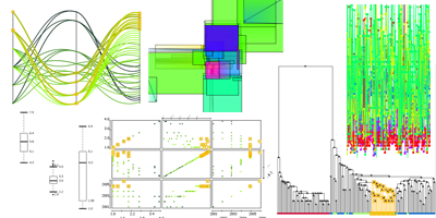
KNIME Interactive Views
One of my responsibilities at KNIME is the design and implementation of interactive views.
KNIME, pronounced [naim], is a modular data exploration platform that allows the user to visually create data flows (often referred to as pipelines).
This article should shortly introduce the views I developed so far and some which are still under construction. I describe the following views:
each with a screenshot and how the information is displayed in each visualization.
As the dataset for this article I used my marks of my studies, which can be viewed here.
In KNIME there is the possibility to assign visual properties to the data throughout the whole workflow. I used a color coding for the marks (in Germany a 1 is the best, 4 is worst but still passed) ranging from dark green for 4 and light green for 1.
Additionally, I used different shapes: a diamond for all my courses in my bachelor studies, a circle for my courses of my master studies at the Technical University of Cottbus and a triangular for my master courses at the University of Konstanz.
Another advantage of KNIME is the possibility to highlight some data points. What we call highlighting is also often referred to as Linking&Brushing. The visual properties of highlighted data points is on the one hand the orange color and on the other hand the rectangle around the data point, clearly identifying it as highlighted. Linking&Brushing enables the user to select some points of interest in one view and highlight them. Then this information is propagated to all other related views, such that the points of interest are clearly identifiable in each view. I highlighted all marks achieved at the University of Konstanz.
Scatterplot (with a linear regression line):
This view plots the data with the marks ranging from 1 to 4 at the y axis (vertically) and the years ranging from 2001 to 2006 on the x axis (horizontally).
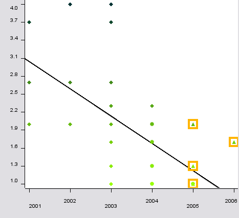
As one can see at the regression line, the marks definitively improved during my studies. The different visual properties like color and shape are also visible.
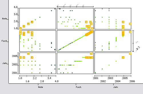
Scatterplot Matrix:
There are some problems related to the scatterplot. First, if several data points share the same coordinate it is not visible to the user. This problem is also known as overplotting Second, a scatterplot can always use only two dimensions. If the data has more dimensions (attributes) the user must constantly switch the displayed dimensions in order to understand the data.
The use of a scatter matrix overcomes the second problem (but is also restricted to low dimensional data). All dimensions of the dataset are plotted as a matrix, where each attribute is plotted against each other.
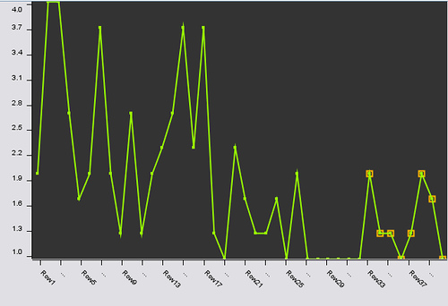
Line Plot:
The line plot is a very well known view. In contrast to a scatterplot or parallel coordinates not the values of one data point (instance or row of the data) are plotted but the values of one attribute (or column). Thus, the color and shape information are not available, since they describe the values of one data point. Here are all marks plotted as they occur in the data set from left to right (I ordered the data set in advance so they are also plotted from 2001 to 2006).
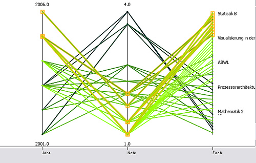
Parallel Coordinates:
Parallel Coordinates are an attempt to overcome the problem of displaying data with more than 2 (or 3 if you want) dimensions. Each attribute is displayed as a vertical line, ranging from the lowest value of that attribute to the highest. As one can see the axis representing the year attribute (which ranges from 2001 – 2006) is as long as the axis of the mark attribute (1- 4). Each data point is plotted as a line. The line intersects the axis at the values the data point has in this dimension. If one looks, for example, at the two 4 marks at the top, one can follow the line and see that one was obtained in 2002 and one in 2003.
Since the highlighted lines represent my marks obtained at the University of Konstanz one can easily see, that here the marks range from 1.0 to 2.0 (with the intermediate steps of 1.3 and 1.7).
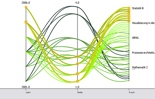
One problem related to parallel coordinates is that if several lines intersect at one point of one axis it is hard to follow the lines after the intersection (if the are not color coded). One possibility to overcome this is to plot the lines as curves. While this is not always true one can see when looking at the 2.0 (the highest of the highlighted points), that one can clearly distinguish the curves coming from 2001, 2002 and 2005.
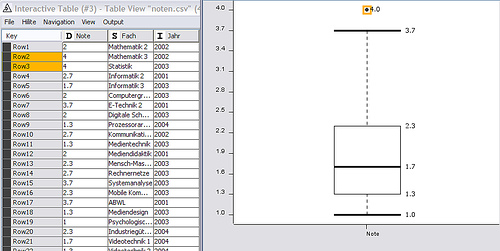
Box Plot:
The box plot (or box and whisker plot) displays robust statistics (you may also be interested in my article about box plots). Why robust? In contrast to the mean, which is calculated as the sum of the values divided by the number of values, the median is determined by sorting the data and then choosing the one in the middle (if the number of data points is odd the mean of the two data points left and right the middle is taken).
A simple example should make the idea clear. The mean of my marks is 1.8825. If the marks are sorted, they look like:
1.0, 1.0, 1.0, 1.0, 1.0, 1.0, 1.0, 1.0, 1.0, 1.0, 1.3, 1.3, 1.3, 1.3, 1.3, 1.3, 1.3, 1.3, 1.7, 1.7, 1.7, 1.7,
2.0, 2.0, 2.0, 2.0, 2.0, 2.0, 2.0, 2.3, 2.3, 2.3, 2.7, 2.7, 2.7, 3.7, 3.7, 3.7, 4.0, 4.0.
All together 40 marks and the one in the middle (the 20th) is a 1.7, thus the median of my marks is 1.7 in contrast to the mean of 1.8825. For the sake of this example, assume the two 4.0s were two 5.0s. Beside the fact that then I would have failed the courses, the mean of my marks would then be 1.9325. The median remains 1.7. This is meant by robust statistics: it is less sensible to outliers.
However, a box plot displays much more information. Here is the list of parameters which are necessary to calculate:
- lower quartile Q1 (which is the value at the lower 1/4 of the data)
- upper quartile Q3 (which is the value at the 3/4 of the data)
- the interquartile range (IRQ), which is the range between the two quartiles, thus Q3 – Q1
- the minimum value: the smallest observation which is not smaller than 1.5 * Q1
- the maximum value: the largest observation which is not larger than 1.5 * Q3
- the mild outliers: all values between 3*Q1 - 1.5*Q1 and 1.5*Q3 – 3*Q3
- extreme outliers: all values smaller than 3*Q1 or larger than 3*Q3
Now we are ready to draw the box:
The bold line in the middle of the box is the median, the lower border of the box is Q1, the upper border Q3. The whiskers (the horizontal lines outside the box) display the values which are closest to 1.5* Q1 or 1.5*Q3 but still are inside this interval. All values outside this interval are mild outliers and are plotted with a dot. Extreme outliers may be displayed using a different shape. As one can see: my worst marks are definitively outliers ;0)
Dendrogram:
A dendrogram displays the result of a hierarchical clustering. This starts with every data point as one cluster. In the next step those two data points (i.e. clusters) are combined, which are closest. This is done for all remaining data points. In the next steps those clusters are combined which have the closest distance (of course, there are several methods to measure the distance of two clusters – but this goes beyond the scope of this article). Eventually, all data points are in one cluster.
A dendrogram displays all results of the process of hierarchical clustering. At the bottom there are all data points and at the top is the super cluster which contains all data points. Each combination of two clusters is displayed as two vertical lines starting at the clusters, connected by a horizontal line. The height of this horizontal line corresponds to the distance between the combined clusters.
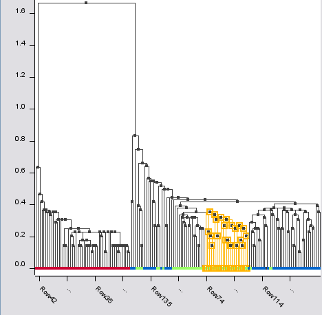
Since my marks are more or less one dimensional, I used for the hierarchical clustering the Iris data set.
Rule 2D View
I also implemented a chart for rules. Rules are a common classification technique in Knowledge Discovery. As with most classification tasks the algorithm is trained with already labeled data. When the performance is good enough it is able to classify unseen instances based on the rules learned from the training data.
Basically, rules consist of an interval for each dimension and the referring label, saying if the data point lies within this interval it belongs to this and that class.
A problem related to this kind of rules are those data points located at the border of the intervals. If they are close to the border but outside – are they really not instances of this class? If they are close to the border but inside the interval – do they belong as much to the class as those points in the center of the interval.
A well-known technique to model uncertainty, i.e. the data points close to the border belong to that class to a certain degree. Then a fuzzy rule consists of an area, where the degree is equal to 1 (called the core), and an area where the degree lies between 0 and 1 (called the support). A one-dimensional fuzzy rule is typically depicted like this:
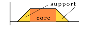
Since I wanted to show 2 dimensional rules, the above shown rule is considered to be seen from top, which results in:
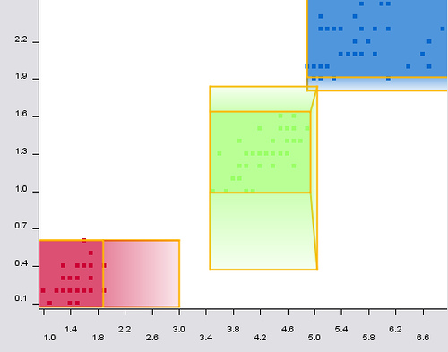
You can see the core area as a rectangle and the support area as the regions where color fades such as the degree of memberships decreases. In oder to better understand the rules the data points they are covering are also displayed and are still visible under the rules.
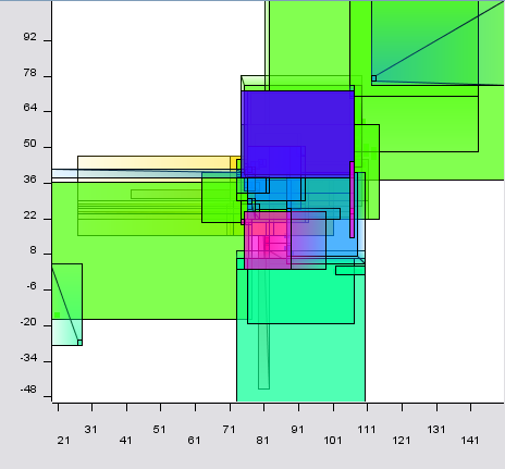
A more complex system of fuzzy rules may look like this:
I a interested in predicting
I a interested in predicting the activity of a set of compounds with a training set and descriptors associated with them.I have 10 descriptors and am interested in developing a modelfor a test set and predcit activity using knime.Kindly suggest
Hi Anand, it is of course
Hi Anand,
it is of course possible to build a predictive model in KNIME. I don't know which kind of model you are interested in: decision tree, neural network, etc.
In KNIME you would read in your training set connect it to a learner (e.g. decision tree learner), then connect the test set with the referring predictor (e.g. decision tree predictor) which would append with an additional column to your test set containing the predicted activity.
By the way: if the activity is not categorical ("yes" or "no") but a number you can't use a decision tree but some other learning models (regression, neural network, etc.)
Hope that helps. For further questions I would suggest to go to the KNIME forum directly and ask there your questions.
Thanks for your interest!
Fabian
I tried to use Knime to
I tried to use Knime to connect to my database.
However, you have only one choice for the drive:
sun.jdbc.odbc.JdbcOdbcDriver
and provide the following:
Database URL
User Name
Password
Since I am using DHCP, it does not work in my labtop.
I have sqlDeveloper and TOAD installed in my computer that use either Oracle.jdbc.OracleDriver or oracle.jdbc.driver.OracleDriver. Both work in my computer.
I tried to create a node but it seems that the free version
does not have this option.
Any comment?
John
Hi John, All database nodes
Hi John,
All database nodes in KNIME allow the registration of additional database drivers from file (jar or zip), see the node dialog's "LOAD" button. As soon as you have selected the driver file, the list will be updated with all SQL compatible drivers. Note, other KNIME user- or developer-related questions may also be posted into our forum at www.knime.org
Regards, Thomas
Post new comment